Concentrated liquidity
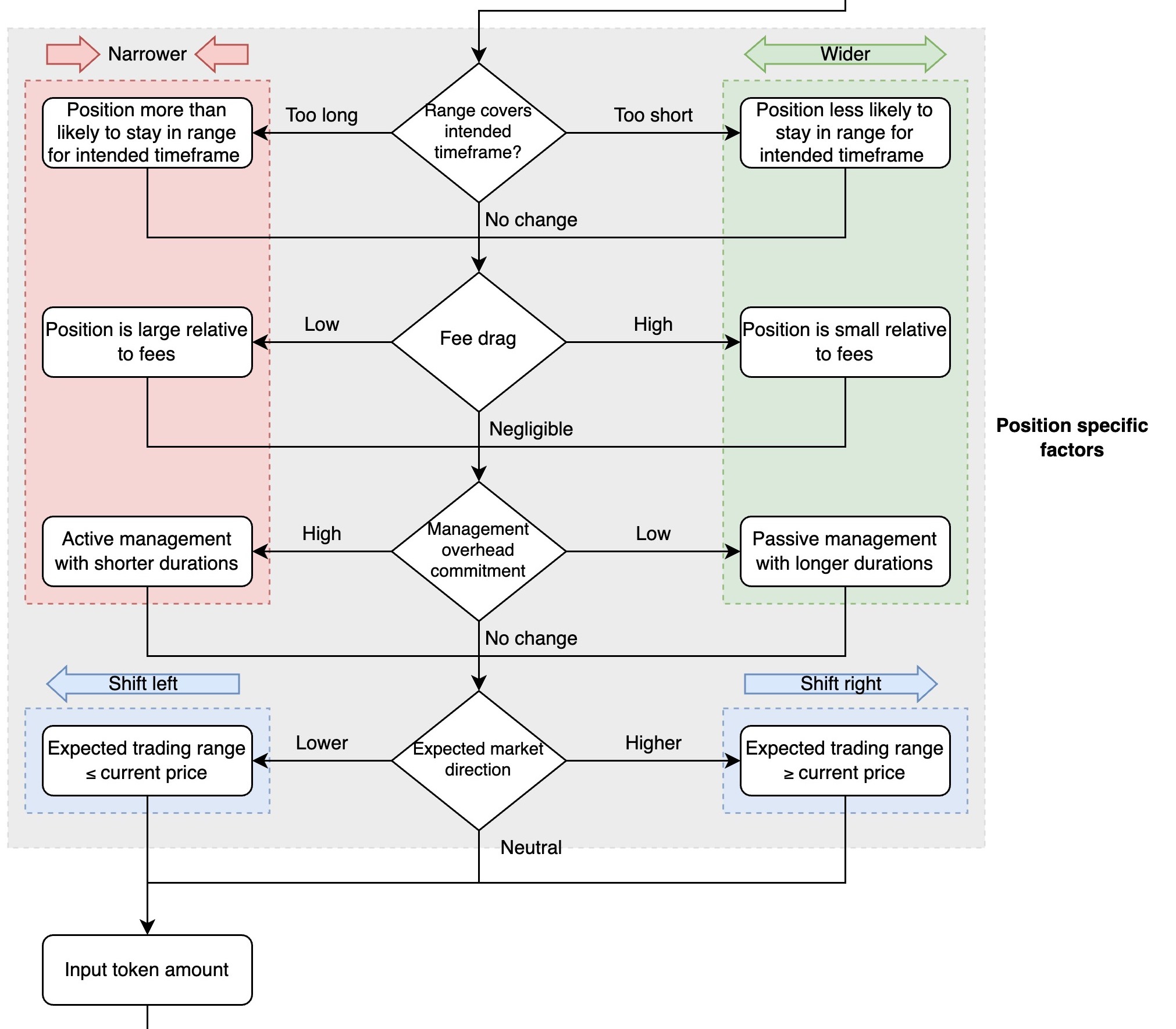
 A LPs returns are heavily dependent on the [position range selected](https://github.com/KyberNetwork/kyberswap-documentation/blob/main/reference/legacy/kyberswap-elastic/concepts/broken-reference/README.md) for [concentrated liquidity](https://docs.kyberswap.com/reference/legacy/kyberswap-elastic/concepts/concentrated-liquidity) protocols such as KyberSwap Elastic. To help you maximize your potential returns, [KyberSwap Insights](https://blog.kyberswap.com/learn/insights-en/) has created a simple flow diagram which walks you through each of the key decision points when determining a position range which best suites your risk-adjusted return preferences.
View and interact with the full diagram in greater detail [here](https://blog.kyberswap.com/choosing-the-best-range-to-maximize-lp-returns-flow-chart/).
{% endhint %}
## The evolution of AMMs
### Basic price curve with infinite price range
The basic AMM started by implementing a standard constant product curve (`x*y=k`)whereby liquidity was uniformly distributed across an infinite price range (i.e. 0 → ∞). While this supported trades across all possible price ranges, majority of the capital was left unutilized as trades for most tokens would usually be within a much narrower price range. This was especially so for more correlated pairs such as stablecoin pairs (i.e. USDC/USDT, DAI/USDC, etc.) or wrapped token pairs (i.e. wstETH/ETH, HBTC/WBTC, etc.) where price ratios rarely diverged.
Consequently, suboptimal capital allocation resulted in greater slippage risks as there was less liquidity supporting widely traded price ranges. With fewer trades, LPs would also receive less fees while simultaneously having to bear the opportunity cost of locked but unutilized funds. The cumulative result of the above was that markets would also tend to be more volatile as limited liquidity meant that trades against smaller pools would result in significant price impacts which might kickstart a vicious cycle.
### Modified price curve with infinite price range
As all trades against an AMM takes place against the specified price curve, it was possible to improve upon the capital efficiency of the basic constant product curve by modifying the price curve equation. The most well-known variant of this approach is Curve's StableSwap which introduced a linear invariant (`x+y=C`) to the constant product curve. This effectively modified the price curve to better support trades between super-stable pairs which tended to trade very closely to a 1:1 ratio.
This price curve modification enabled trades against a balanced pool to have minimal price impact while still allowing the pool to rebalance itself through exponential price growth in times of extreme volatility. As a result of better support for stable pair swaps, more trades could be incentivized through the lowering of trading fees as the corresponding impermanent loss risks were also minimized. This worked great for super stable pairs but was not suited for token pairs which tended to trade at various price ratios for extended periods of time. Moreover, while greatly minimized, capital was still being deployed to support price extremes.
### Modified price curve with bounded price range
Keeping with the core design of the earlier version, it was discovered that liquidity could be better utilized if pools were created with a more tightly bounded price curve. For example, instead of uniformly distributing liquidity across a 0 → ∞ range, the lower and upper bound of the range should approximate the the price interval which the token pair regularly trades at. This meant that capital efficiency was greatly amplified the narrower the supported price range (i.e. a range of 0.99 → 1.01 instead of 0.9 → 1.1 is roughly 10x more capital efficient).
More liquidity supporting a narrower price range also effectively reduced slippage risks as the trade size would have to scale up according to the pool to have the same price impact. Consequently, these modified price curves worked especially well for more stable pairs where the risks of going out of range was minimal. Critically, this bounding of ranges could work hand-in-hand with price curve modifications to significantly increase capital efficiency while generalizing the applicability of this approach for all token pairs. This was the approach which [KyberSwap Classic](https://github.com/KyberNetwork/kyberswap-documentation/blob/main/reference/legacy/kyberswap-elastic/concepts/broken-reference/README.md) took.
While this design enabled liquidity to be better utilized, it was limited in its ability to support multiple liquidity preferences as the price curve had to be fixed at the point of pool creation. This meant that LPs had to choose between adding liquidity to a specific range defined by the pool creator or else create their own pool (which also comes with significantly more gas fees). As such, depending on LP risk preferences, liquidity was likely to be fractured across different pools for the same token pair resulting in less than ideal slippage and trading volume.
### Aggregated price curve with user defined ranges
With each LP having their own liquidity preference, it only made sense that this should be reflected accordingly in the pricing curve. By enabling LPs to add liquidity to their preferred price ranges, each of these positions effectively formed their own user-defined price curve against which trades could be made against. In other words, as long as trades were occurring within the user-defined ranges, their liquidity is utilized in the market making process and hence they will earn trading fees for supporting trades within the particular "tick". Through aggregating all the different positions into a single price curve, it enabled a single pool to support the diversity of LP preferences. This was the design popularized by Uniswap v3 and has come to be known as concentrated liquidity.

Concentrated liquidity

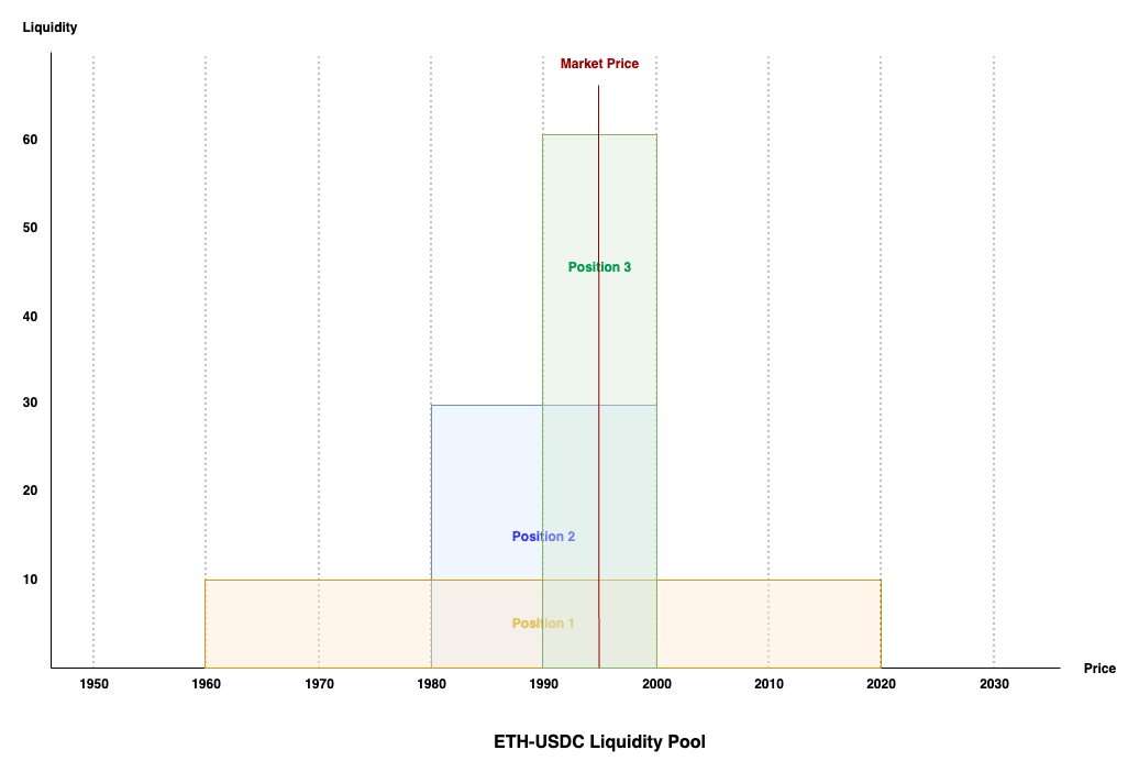
Liquidity concept
| Position | TVL (USD value) | Price Range | Liquidity Contributed |
| 1 | 6,000 | 1,960-2,020 (Width: 60) | 10 |
| 2 | 6,000 | 1,980-2,000 (Width: 20) | 30 |
| 3 | 6,000 | 1,990-2,000 (Width: 10) | 60 |